Word Field Analysis
This guide is also available as a vignette in the R console: vignette(Word-Field-Analysis).
- Word Field Definition
- Single word field
- Multiple Word Fields
- Dictionary Based Distance
- Development over the course of the play
A word field is basically of a list of words that belong to a common theme / topic / semantic group.
For demo purposes (this is really a toy example), we will define the
word field of Love as containing the words Liebe and Herz. In R,
we can put them in a character vector:
wf_love <- c("liebe", "herz")We will test this word field on Emilia Galotti, which should be about love.
data("rksp.0")The core of the word field analysis collecting statistics about a
dictionary. Therefore, we use the function called
dictionaryStatisticsSingle() (single, because we only want to analyse
a single word field):
dstat <- dictionaryStatisticsSingle(
  rksp.0$mtext,         # the text we want to process
  wordfield=wf_love,   # the word field
  column="Token.lemma" # we count lemmas instead of surface forms
)

summary(dstat)
## corpus drama figure x
## test:13 rksp.0:13 angelo :1 Min. : 0
## appiani :1 1st Qu.: 0
## battista :1 Median : 2
## camillo_rota :1 Mean : 3
## claudia_galotti:1 3rd Qu.: 5
## conti :1 Max. :10
## (Other) :7
We can visualise these counts in a simple bar chart:
# remove figures not using these words at all
dstat <- dstat[dstat$x>0,]

barplot(dstat$x,                   # what to plot
        names.arg = dstat$figure,  # x axis labels
        las=3,                     # turn axis labels
        cex.names=0.6,             # smaller font on x axis
        col=qd.colors              # colors
      )
Apparently, the prince is mentioning these words a lot.
Obviously we would want to normalize according to the total number of spoken words by a figure:
dstat <- dictionaryStatisticsSingle(
  rksp.0$mtext,       # the text we want to process
  wordfield=wf_love, # the word field
  normalizeByFigure = TRUE,   # apply normalization
  column = "Token.lemma"
)

# remove figures not using these words at all
dstat <- dstat[dstat$x>0,]

barplot(dstat$x,
        names.arg = dstat$figure,  # x axis labels
        las=3,             # turn axis labels
        cex.names=0.8,     # smaller font on x axis
        col=qd.colors
      )
The function dictionaryStatistics() can be used to analyse multiple
dictionaries at once. To this end, dictionaries are represented as lists
of character vectors. The (named) outer list contains the keywords, the
vectors are just words associated with the keyword.
New dictionaries can be easily like this:
wf <- list(Liebe=c("Liebe","Herz","Schmerz"), Hass=c("Hass","hassen"))This dictionary contains the two entries Liebe (love) and Hass
(hate), with 3 respective 2 entries. Dictionaries can be created in
code, like shown above. In addition, the function loadFields() can be
used to download dictionary content from a URL or a directory. By
default, the function loads this
dictionary
from GitHub (that we used in publications), for the keywords Liebe and
Familie (family).
wf <- loadFields()
names(wf)
## [1] "Liebe" "Familie"
The function loadFields() offers parameters to load from different
URLs via http or to load from plain text files that are stored locally.
The latter can be achieved by specifying the directory as baseurl.
Entries for each keyword should then be stored in a file named like the
keyword, and ending with txt (by default, can be overwritten). See
?loadFields for details. Some of the options can also be specified
through dictionaryStatistics(), as exemplified below.
The following examples use the baseurl
https://raw.githubusercontent.com/quadrama/metadata/ec8ae3ddd32fa71be4ea0e7f6c634002a002823d/fields/,
i.e., a specific version of the fields we have been using in QuaDramA.
baseUrl <- "https://raw.githubusercontent.com/quadrama/metadata/ec8ae3ddd32fa71be4ea0e7f6c634002a002823d/fields/"
wfields <- loadFields(fieldnames = c("Liebe", "Krieg", "Familie", "Ratio", "Religion"),
                      baseurl = baseUrl)
dstat <- dictionaryStatistics(
rksp.0$mtext, # the text
fields = wfields,
names = TRUE, # use figure names (instead of ids)
normalizeByFigure = TRUE, # normalization by figure
normalizeByField = TRUE, # normalization by field
column = "Token.lemma" # lemma-based stats
)
colnames(dstat)## [1] "corpus" "drama" "figure" "Liebe" "Krieg" "Familie"
## [7] "Ratio" "Religion"
The variable dstat now contains multiple columns, one for each word
field.
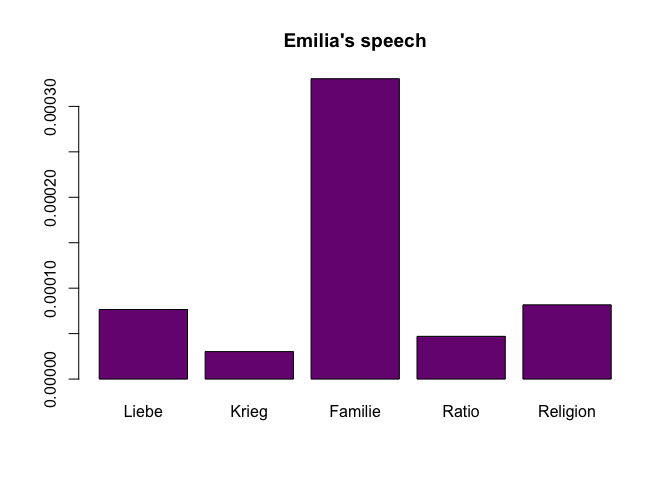
We can now display the distribution of the words of a single figure over these word fields:
barplot(as.matrix(dstat[9,4:8]), # we select Emilia's line
        main="Emilia's speech",    # plot title
        col=qd.colors             # more colors
        )
… but we can also analyse who uses words of a certain field how often
barplot(as.matrix(dstat$Liebe),
        main="Use of love words", # title for plot
        beside = TRUE,            # not stacked
        names.arg = dstat[[3]],  # x axis labels
        las=3,                    # rotation for labels
        col=qd.colors,            # more colors
        cex.names = 0.7           # font size
        )
Technically, the output of dictionaryStatistics() is a data.frame.
This is suitable for most uses. In some cases, however, it’s more suited
to work with a matrix that only contains the raw numbers (i.e., number
of family words). Calculating character distance based on dictionaries,
for instance. For these cases, the function offers a parameter asList.
If it is set to TRUE, the function returns a list with four to six
components. The first three components (corpus, drama, figure,
Number.Act, Number.Scene) contain meta data, while the fourth
component (mat) contains the values as a matrix.
You typically want to assign rownames to this matrix. If you’re studying individual characters, their name might be a good idea.
dsl <- dictionaryStatistics(rksp.0$mtext,
                            fields = wfields,
                            normalizeByFigure=TRUE,
                            asList=TRUE)
dsl$mat
## Liebe Krieg Familie Ratio
## angelo 0.001474926 0.002949853 0.002949853 0.007374631
## appiani 0.006178288 0.004413063 0.009708738 0.006178288
## battista 0.000000000 0.000000000 0.009852217 0.000000000
## camillo_rota 0.009433962 0.009433962 0.000000000 0.047169811
## claudia_galotti 0.005147403 0.004679457 0.013570426 0.004211511
## conti 0.013089005 0.000000000 0.005235602 0.002617801
## der_kammerdiener 0.000000000 0.000000000 0.000000000 0.000000000
## der_prinz 0.005222402 0.002881325 0.005042319 0.003781740
## emilia 0.006347863 0.003385527 0.023698688 0.004655099
## marinelli 0.006537102 0.003180212 0.009363958 0.004063604
## odoardo_galotti 0.003825780 0.004414361 0.015303119 0.006180106
## orsina 0.005064146 0.002700878 0.005739365 0.004726536
## pirro 0.000000000 0.000000000 0.008196721 0.002732240
## Religion
## angelo 0.0014749263
## appiani 0.0000000000
## battista 0.0000000000
## camillo_rota 0.0000000000
## claudia_galotti 0.0028076743
## conti 0.0000000000
## der_kammerdiener 0.0000000000
## der_prinz 0.0019809112
## emilia 0.0038087177
## marinelli 0.0010600707
## odoardo_galotti 0.0029429076
## orsina 0.0006752194
## pirro 0.0027322404
Every character is now represent with five numbers, which can be
interpreted as a vector in five-dimensional space. This means, we can
easily apply distance metrics supplied by the function dist() (from
the default package stats). By default, dist() calculates Euclidean
distance. The data
structure here is now similar to the one in the weighted configuration
matrix, which means everything from this
vignette can be applied here.
cdist <- dist(dsl$mat)
cdist
## angelo appiani battista camillo_rota
## appiani 0.008576233
## battista 0.010727547 0.009789698
## camillo_rota 0.041230126 0.042548483 0.050000566
## claudia_galotti 0.011876731 0.005272340 0.009372194 0.045589856
## conti 0.013176341 0.009995957 0.014124025 0.045985347
## der_kammerdiener 0.008725781 0.013786849 0.009852217 0.049020306
## der_prinz 0.005620639 0.005890912 0.008771328 0.044413377
## emilia 0.021616936 0.014616078 0.016722984 0.049292418
## marinelli 0.008829181 0.002713518 0.008409666 0.044659307
## odoardo_galotti 0.012800639 0.006744784 0.010520928 0.044493260
## orsina 0.005327082 0.004742606 0.008523610 0.043580472
## pirro 0.007844699 0.008903535 0.004203682 0.047194792
## claudia_galotti conti der_kammerdiener der_prinz
## appiani
## battista
## camillo_rota
## claudia_galotti
## conti 0.012839727
## der_kammerdiener 0.016067651 0.014338287
## der_prinz 0.008765600 0.008689166 0.008900903
## emilia 0.010339048 0.020407039 0.025486492 0.018806504
## marinelli 0.004994935 0.008561460 0.012576478 0.004628360
## odoardo_galotti 0.002951752 0.015099654 0.017752832 0.010782503
## orsina 0.008370175 0.008766389 0.009416830 0.001772273
## pirro 0.008914242 0.013695566 0.009061816 0.006869623
## emilia marinelli odoardo_galotti orsina
## appiani
## battista
## camillo_rota
## claudia_galotti
## conti
## der_kammerdiener
## der_prinz
## emilia
## marinelli 0.014610523
## odoardo_galotti 0.008998903 0.007223067
## orsina 0.018288736 0.004015547 0.010158260
## pirro 0.017231492 0.007666719 0.009826303 0.006869313
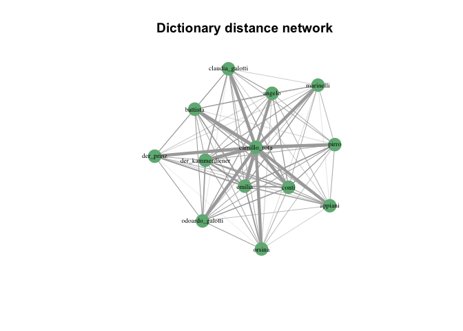
In particular, we can show these distances in a network:
require(igraph)## Loading required package: igraph
## Warning: package 'igraph' was built under R version 3.4.4
## Loading required package: methods
##
## Attaching package: 'igraph'
## The following objects are masked from 'package:stats':
##
## decompose, spectrum
## The following object is masked from 'package:base':
##
## union
g <- graph_from_adjacency_matrix(as.matrix(cdist),
                                 weighted=TRUE,     # weighted graph
                                 mode="undirected", # no direction
                                 diag=FALSE         # no looping edges
                                )

# Now we plot
plot.igraph(g,
            layout=layout_with_fr,       # how to lay out the graph
            main="Dictionary distance network",  # title
            vertex.label.cex=0.6,         # label size
            vertex.label.color="black",   # font color
            vertex.color=qd.colors[5],    # vertex color
            vertex.frame.color=NA,        # no vertex border
            edge.width=E(g)$weight*100    # scale edges according to their weight
                                          # (since the distances are so small, we multiply)
) 
Since version 2.0 of this package, we can also count word fields by
segment, i.e., by act or scene in a play. To do that, we add the
parameter segment="Act" when we call the function
dictionaryStatistics(). With the function individualize(), we can
then re-organize this output so that each character has its own list.
dsl <- dictionaryStatistics(rksp.0$mtext,
                            fields = wfields,
                            normalizeByFigure=TRUE,
                            asList=TRUE,
                            segment="Scene")

dsl <- regroup(dsl)
We can now easily plot the theme progress over the course of the play:
matplot(dsl$marinelli$mat,type="l",col="black")
legend(x="topleft",legend=colnames(dsl$marinelli$mat),lty=1:5)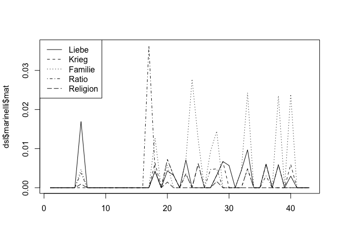
Or cumulatively add up the numbers:
mat <- apply(dsl$marinelli$mat,2,cumsum)
matplot(mat,type="l",col="black")

# Add act lines
al <- rle(dsl$marinelli$Number.Act)
abline(v=cumsum(al$lengths[-1]))

legend(x="topleft",legend=colnames(mat),lty=1:5)